Quickly format a cell as “Currency”

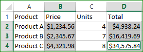
Cells are normally formatted as “General”, which means there is no special formatting applied to the numbers typed into cells. If you type 123.45 then 123.45 is what you’ll see. Look at this simple table below:

You can quickly format the Price and Total columns as Currency by selecting all the relevant cells and pressing Ctrl+Shift+$, conveniently placing a Dollar sign before each number, formatting it with two decimals and adding a thousands separator.

Other currencies

But what if your country’s currency is not the good ol’ dollar? What if you would like Excel to default to British Pound, or South African Rand or Korean Won, or Japanese Yen?

Well that actually depends on the computer that you are working on.  You can change it in a matter of seconds by adjusting your Regional Settings (on a Windows PC).

Step 1: Change the default number format for currency in Control Panel.

You can get there quickly by pressing the Win key (looks like the Windows logo). This opens your Start menu. Now type the words number format and the relevant Control Panel item will pop up (Change the date, time or number format):

This will take you to the Region and Language settings. Here you can either pick a different Format to change everything at once to match your region (date, time, currency, keyboard layout, etc.) Or…. you can just change the Currency number format by selecting Additional Settings, and updating the currency symbol in the Currency tab.

Then pick a new currency symbol:

Step 2: Close and re-open Excel.

The currency shortcut (Ctrl+Shift+$) should now pick up your new currency symbol!

More on Number Formats

You can manually edit number formats to suit your specific needs by entering a Custom number format. E.g. you may want to use brackets for negatives instead of a negative sign. Or, you may want to show numbers as thousands, e.g. $12,345,723 should be shown as $12,346.

After selecting a cell containing a number, go to the Format Cells dialog (shortcut Ctrl+1) and select Custom.

The custom format field consists of four parts: positive numbers, negative numbers, text and zero. The four fields are separated by a semicolon. If you find it daunting to edit this field, you may want to copy the formatting from a cell that is already formatted the way you like it.

You can save frequently used formats in a worksheet, where you can just copy and paste it into the Custom field above when required. Below is an example:

Download the .xlsx file here!

You could create new Cell Styles using your desired formatting, but I’ve found that a cheat sheet like the one above is handy for quickly cleaning up the formatting of a messy spreadsheet.

You can make it even easier to reach you cheat sheet by pinning it to your Recent Workbooks tab. If you’ve recently opened the workbook it will show up on your Recent Workbooks tab. Click on the little thumbtack on the right to lock the workbook in place. It will now always appear on the Recent Workbooks list, even if you haven’t accessed it recently. You can also do this for other worksheets of course!

Let me know in the comments if anything doesn’t make sense and I’ll do my best to clarify.

Now go format some numbers!